Introduction
This vignette gives a detailed account on the workflow of UniPath tool for analyzing single cell expression data and single cell open chromatin profiles in pathway domain. UniPath is a steadfast statistical method for getting important biological insights from single cells characterized in terms of pathway activity scores and studying temporal dynamics. UniPath is a scalable platform allowing pre-processing and analysis of thousands of single cells by exploiting heterogeneity among cells and uncovering biologically relevant pathways. UniPath can help users with accurate identification of cell types, signaling pathways and doublet cells. Besides these, the user can also perform clustering and pseudo temporal ordering of single cells in pathway space. This may allow the analysis of relevant pathways and genes on single cell lineage transitions or potency.
Installation
To install the package use following command (may work well with R version 3.5.1).
library(devtools)
install_github("reggenlab/UniPath")
User can also install package using . tar.gz file. Click here to download UniPath_0.1.0.tar.gz file.
Use following credentials to download:- Username: reggen , Password: unipath@123
R CMD INSTALL UniPath_0.1.0.tar.gzFor details about each and every function in UniPath Package download the manual(click here).
In case of installation issues, check for the dependencies associated with the package. They can be installed from the following links:
For other applications of UniPath, we suggest users to install DrImpute, ggplot2 and reshape2 packages. Also, we have used EmpiricalBrownsMethod package from R.
Usage and workflow
For details about each and every function in UniPath Package download the manual(click here).
For single cell data analysis, UniPath package comes with a precompiled mouse and human null model data. Also, for transformation of single cell gene expression data into pathway or gene-set enrichment scores, the package contains pathway annotation and gene set marker files.
The analysis of single cells starts by loading following data files:
• Mouse/human null model data matrix
• Gene set maker file
• Gene expression matrix (Where genes should be in rows and samples/cells should be in columns). Ensure that genes are set as row names of the matrix.
We have used mouse lung data (GSE52583, Treutlein, Barbara et al.) consisting of 23007 genes and 194 cells for this tutorial. For example:
library(UniPath)
##Load all data files
data("mouse_null_model")
data("c5.bp.v6.0.symbols")
data("GSE52583_expression_data")
For tutorial purpose, in-built data is provided but users can also read or load their own input data files.
Conversion of gene expression FPKM value to P-value
Next, we transformed gene FPKM values to p-values using individual cell’s mean and standard deviation based on the assumption that non-zero FPKM value in cell follows log normal distribution.
##Converting mouse null data into p-values
Pval = binorm(mouse_null_data)
##Converting gene expression data into p-values
Pval1 = binorm(expression_data)
Combining of P-values
To take into account interdependency of p-values, we used browns method to combine p-values of genes in gene sets using combine() function for individual cells. We are using pathway annotation file having 4436 gene sets for transforming data into pathway space.
##Combining of p-values for null model data matrix
combp_ref = combine(c5.bp.v6.0.symbols,mouse_null_data,rownames(mouse_null_data),Pval)
##Combining of p-values for gene expression data matrix
combp = combine(c5.bp.v6.0.symbols,expression_data,rownames(expression_data),Pval1)
Adjusting of P-values
To avoid unwanted effects of background housekeeping genes and for highlighting cell type specific gene-set activities, we adjust p-values using null model. This adjusted p-value matrix is referred to as pathway scores.
scores = adjust(combp,combp_ref)This will return a list of three matrices one with adjusted p-values, second one with adjusted raw p-values and third one is log transformed adjusted p-values.
In a similar way, we can transform human gene expression into pathway scores using the human null model as shown in the example below. We have used human lung cancer expression data here which is a part of package.
library(UniPath)
data("human_null_model")
data("c5.bp.v6.0.symbols")
data("lungcancer_expression")
Pval = binorm(human_null_data)
combp_ref <- combine(c5.bp.v6.0.symbols,human_null_data,rownames(human_null_data),Pval)
Pval1 = binorm(expression_matrix)
combp <- combine(c5.bp.v6.0.symbols,expression_matrix,rownames(expression_matrix),Pval1)
scores = adjust(combp,combp_ref)
Single cell ATAC-seq
UniPath transforms single cell open chromatin to pathway enrichment scores by highlighting cell type specific enhancers through normalization of profiles by global or local accessibility scores.
Global accessibility scores
To control for sequencing depth and dropout rate, firstly we highlight cell type specific enhancer by dividing scATAC-seq profiles by their global accessibility scores. For global accessibility scores computation, bulk ATAC-seq peaks have been curated. Using this combined/reference peak list, global accessibility scores are calculated for each genomic site based on the proportion of samples, the site was detected as open chromatin peak. Global accessibility scores for test dataset is calculated using global_access() function. For this tutorial, we have used human scATAC-seq keratinocytes differentiation data at three time points from GEO: GSE116248 study. Global accessibility scores for this dataset is calculated using global_access() function as shown in example below. User has to input genomic coordinate or peak file for this dataset along with the reference peaks list and human global accessibility scores.These data files are loaded from extdata folder of UniPath.
##First set up a working directory
setwd(system.file("extdata", package="UniPath"))
globalaccess = global_access("GSE116248_peaks.txt","reference_peaks_human.txt","global_accessibility_score_human.csv")
User can also perform imputation of scATAC-seq data as shown below. Imputation improves the quality of data, thus it's a user choice. For this tutorial, we have used Drimpute for imputation which is time consuming task. Therefore, imputed keratinocytes data is a part of this package. Raw count file used for imputation used below as well as other additional files can be downloaded from the link Click here to download GSE116248_counts.csv file.
imputed_count = drimpute("GSE116248_counts.csv")Conversion of scATAC-seq profiles into pathway enrichment scores
UniPath provides two methods for normalization of scATAC-seq profiles in each cell, one is global accessibility score and other is using local accessibility score . After normalizing scATAC-seq profiles, peaks having high normalized counts are considered as foreground and all peak set is used as a null or background model. Then, the nearest gene within 1MBp of the peak is considered for conversion into pathways enrichment scores using either hypergeometric test or binomial test. User can use same background file for all scATAC-seq datasets but for foreground file user require to install perl in the system and then use nearest_gene function to create forgeground file as shown below. This function takes four arguments: First is nearest gene perl script, second is peak list then human reference genome file and last one is output file name. This is followed by system calling of perl script.
cmd = nearest_gene("nearestGenes.pl","GSE116248_peaks.txt","refseq-hg19.txt","GSE116248_foreground")
##system call
system(cmd)
data("c2.cp.v6.1.symbols")
scores = runGO(c2.cp.v6.1.symbols,"background_human","GSE116248_imputed_count.csv",method=1,"globalaccess","GSE116248_foreground",promoters = FALSE)
Above function will return list of two dataframes containing pathway scores based on hypergeometric and binomial test respectively. After conversion of scRNA-seq and scATAC-seq into pathway scores, user can perform number of downstream analysis to get biologically useful insights which are discussed in below sections.
In a similar way, we can tranform mouse single cell ATAC-seq profiles using mouse global accessibility scores.
Pseudo temporal ordering
In UniPath, for pseudo temporal ordering we first perform the initial level of classification of cells using hierarchical clustering approach on pathway scores matrix. Then in order to avoid wrong ordering of cells, we compute the top k nearest neighbor (KNN) index for each cell. And based on these indices and belongingness of the cells to same class as well number of times top KNN of a particular class is occurring in other class, we perform two levels of distance shrinkage for every cell pair. Using this shrunk distance matrix, minimum spanning tree is plotted. We have used 4 clusters for mouse lung data since there are 4 types of cells and k=5 for top k nearest neighbor computation.
Example of scRNA-seq data
##Performing hierarchal clustering on pathway score matrix
##User has to specify number of classes
distclust = dist_clust(scores$adjpvalog,4)
dist = distclust$distance
clusters = distclust$clusters
##Specifying number of top k nearest neighbor
index = index(scores$adjpvalog,5)
###getting cluster number for each of the KNN for individual cell
KNN = KNN(scores$adjpvalog,index,clusters)
##Two level shrinkage of distance matrix based on clusters and KNN
class = class1(clusters,KNN)
distance = distance(dist,class,clusters)
##Computation of MST on shrinked distance matrix
corr_mst = minimum_spanning_tree(distance)
User has to define the cell labels or groups along with the colors to be plotted on minimum spanning tree. It can be defined as shown below or user can input their cell labels.
##Plotting of MST
vertex_color = c("red","green","blue","yellow")
cell_labels = data.frame(c(rep("E18.5",82),rep("E14.5",44),rep("Adult",46),rep("E16.5",23)))
UniPath::mst.plot.mod(corr_mst, vertex.color = vertex_color[cell_labels[,1]],mst.edge.col="black",bg="white",layout.function="layout.kamada.kawai",v.size = 2, e.size=0.005,mst.e.size = 0.005)
legend("top", legend = sort(unique(cell_labels[,1])), col = vertex_color,pch=20, box.lty=0,cex=0.6,pt.cex=1.5,horiz=T)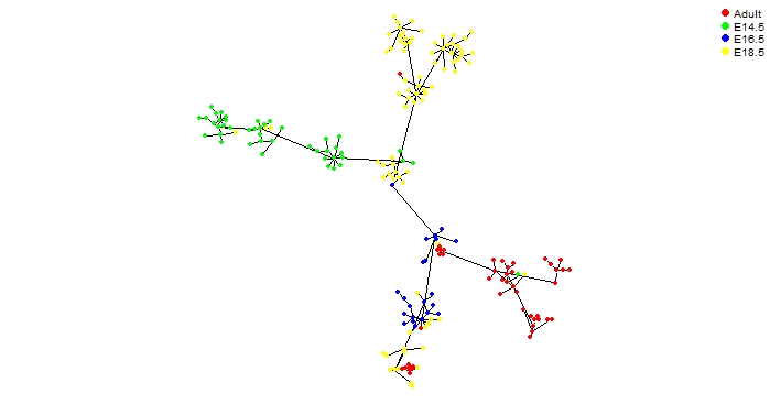
Considering mouse lung developmental data from Treutlein, Barbara et al., we performed pseudo temporal ordering to trace developmental hierarchy of lung from epithelial cells at 4 different stages.
Another example is of scRNAseq time course differentiation data of human embryonic stem cells from study Chu et al (GEO ID: GSE75748). We have included precompiled pathway scores of this study, which can be directly used for performing pseudo temporal ordering as shown in example below.
library(UniPath)
data("GSE75748pathwayscores")
distclust = dist_clust(GSE75748pathwayscores,6)
dist = distclust$distance
clusters = distclust$clusters
index = index(GSE75748pathwayscores,4)
KNN = KNN(GSE75748pathwayscores,index,clusters)
class = class1(clusters,KNN)
distance = distance(dist,class,clusters)
corr_mst = minimum_spanning_tree(distance)
vertex_color = c("yellow","Red","green","blue","black","magenta")
cell_labels  = data.frame(c(rep("0h",92),rep("12h",102),rep("24h",66),rep("36h",172),rep("72h",138),rep("96h",188)))
set.seed(100)
UniPath::mst.plot.mod(corr_mst, vertex.color = vertex_color[cell_labels[,1]],mst.edge.col="black",bg="white",layout.function="layout.kamada.kawai",v.size = 3,e.size=0.005,mst.e.size = 0.005)
legend("topright", legend = sort(unique(cell_labels[,1])) , col = vertex_color,pch=20, box.lty=0,cex=1,pt.cex=2,horiz=F)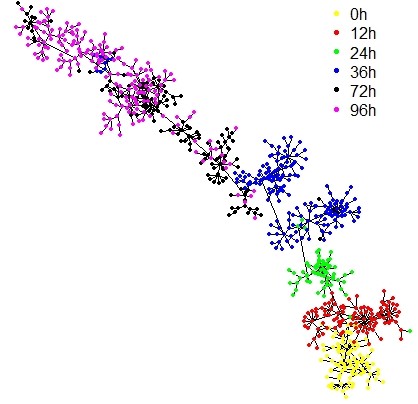
Example for scATAC-seq data
adjpva = -log2(scores$hypergeometeric+.0001)
distclust = dist_clust(adjpva,3)
dist = distclust$distance
clusters = distclust$clusters
index = index(adjpva,5)
KNN = KNN(adjpva,index,clusters)
class = class1(clusters,KNN)
distance = distance(dist,class,clusters)
corr_mst = minimum_spanning_tree(distance)
vertex_color = c("red","green","blue")
cell_labels = data.frame(c(rep("0days",96),rep("3days",95),rep("6days",97)))
UniPath::mst.plot.mod(corr_mst, vertex.color = vertex_color[cell_labels[,1]],mst.edge.col="black",bg="white",layout.function="layout.kamada.kawai",v.size = 3,e.size=0.005,mst.e.size = 0.005)
legend("topright", legend = sort(unique(cell_labels[,1])) , col = vertex_color,pch=20, box.lty=0,cex=1,pt.cex=2,horiz=F)
Above figure shows keratinocytes differentiation at 3 different time points.
Other beneficial features of using UniPath
Clustering and cell detection
Clustering and classification of cell types is a common task in analyzing single cell data. It helps in the annotation of new and rare cell type classes. Mostly this is done in gene expression space but UniPath introduced an approach to perform these tasks using pathway scores. Pathway scores helped us in cell annotation of unknown cell types along with detection of rare cell classes.
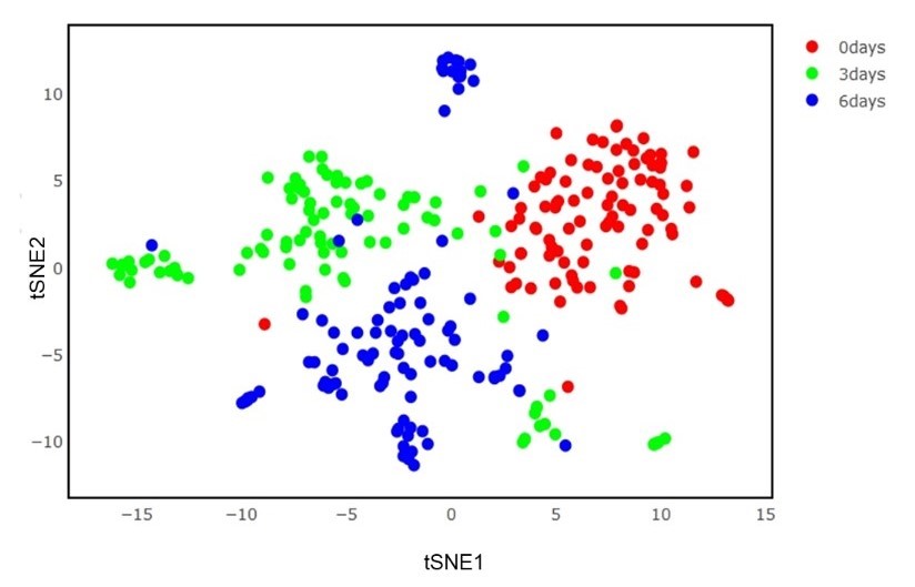
Above plots shows the separation of three classes in pathway space.
UniPath can also help in cell detection based on cell specific gene marker sets which are available in this package. Considering data from study id GSE81861, we have computed gene set enrichment scores using cell type specific marker file as shown in example below.
library(UniPath)
data("human_null_model")
data("GSE81861")
data("human_markers")
Pval = binorm(human_null_data)
combp_ref = combine(human_markers,human_null_data,rownames(human_null_data),Pval)
Pval1 = binorm(data)
combp = combine(human_markers,data,rownames(data),Pval1)
scores = adjust(combp,combp_ref)
In case of scATAC-seq profiles cell detection, human_markers_scATACseq.RData marker file can be used.
Differential pathway analysis
Generally, differential gene expression analysis is performed to distinguish between different cell populations but UniPath can help in finding differentially expressed pathways among different group of cells. It uses Wilcoxon rank sum test for allowing users to access statistically significant pathways among the group of cells. Here, we are using raw pathway scores of same mouse lung data transformed above for getting differential pathways between adult lung stage and rest of the cells in the example below.
##Use raw p-value data
data = scores$adjpvaraw
##define groups
group = as.matrix(c(rep(2,81),rep(2,44),rep(1,46),rep(2,23)))
wilx = temporaldif(data,group)
This will return a list of 3 containing statistical significance(p-values) for enrichment, Fold change based on mean and Fold change based on median for the defined groups. In UniPath for downstream analysis, median fold change is considered.
Differential cooccurrence pathway analysis
Two cell populations can have differences in multiple ways. UniPath introduced the notion of differential cooccurrence pathway analysis for comparing two cell population. It is meant for studying mechanisms involved in controlling different properties of cells. For this purpose it has a function difcoccur() can be used where user can input pathway scores (raw p-values) and group.
For this tutorial, we have included raw pathway scores for lung cancer data which contains 162 cells. We are finding differentially cooccuring pathways in NSCLC TS cells with respect to Adherent NSCLC cells (81 to 162 cells).
library(UniPath)
##Differential cooccurence in NSCLC  TS cells
##load lung cancer pathway scores data
data("lungCancer_pathway_scores")
##Define NSCLC  TS cells in group 1
group = as.matrix(c(rep(1,80),rep(2,82)))
##Perform differential cooccurence
diff1 = difcoccur(pathwayscores,group)
##Two matrices will be generated
pval_TS = diff1$pval
diff_TS = diff1$dif
Similarly, we can find differentially cooccuring pathways in Adherent NSCLC cells with respect to TS NSCLC cells.
##Differential cooccurence in Adherent(Adh) NSCLC cells
data("lungCancer_pathway_scores")
##Define Adherent NSCLC cells in group 1
group = as.matrix(c(rep(2,80),rep(1,82)))
diff2 = difcoccur(pathwayscores,group)
pval_Adh = diff2$pval
diff_Adh = diff2$dif
For visualization extract relevant cooccuring pathway terms as shown in example below.
##Preprocessing of data in required for dotplot based visualization
##Based on the p-value and difference, we will visualize differential cooccurence using dotplot created using ggplot2
##Extract relevant cooccured pathway terms for TS cell group from both pvalue and difference files
pval_TSpathways = reshape2::melt(pval_TS[c("ST_WNT_BETA_CATENIN_PATHWAY","BIOCARTA_SHH_PATHWAY","KEGG_GLYCOLYSIS_GLUCONEOGENESIS"),c("KEGG_TGF_BETA_SIGNALING_PATHWAY","KEGG_NOTCH_SIGNALING_PATHWAY")])
pval_TSpathways = cbind.data.frame(paste(pval_TSpathways[,1],pval_TSpathways[,2],sep="-"),pval_TSpathways[,3])
diff_TSpathways = reshape2::melt(diff_TS[c("ST_WNT_BETA_CATENIN_PATHWAY","BIOCARTA_SHH_PATHWAY","KEGG_GLYCOLYSIS_GLUCONEOGENESIS"),c("KEGG_TGF_BETA_SIGNALING_PATHWAY","KEGG_NOTCH_SIGNALING_PATHWAY")])
diff_TSpathways = cbind.data.frame(paste(diff_TSpathways[,1],diff_TSpathways[,2],sep="-"),diff_TSpathways[,3])
##Defining group label
TS_group = c(rep("TS",6))

##Combine p-value,difference and group for relevant pathways in TS cells
TS = cbind.data.frame(pval_TSpathways,diff_TSpathways[,2],TS_group)
colnames(TS) = c("Pathways","Pvalue","diff","group")

##Same preprocessing in case of Adh cells as TS cells
##Extracting same pathways from ADh group from comparison with TS cells
pval_Adhpathways = reshape2::melt(pval_Adh[c("ST_WNT_BETA_CATENIN_PATHWAY","BIOCARTA_SHH_PATHWAY","KEGG_GLYCOLYSIS_GLUCONEOGENESIS"),c("KEGG_TGF_BETA_SIGNALING_PATHWAY","KEGG_NOTCH_SIGNALING_PATHWAY")])
pval_Adhpathways = cbind.data.frame(paste(pval_Adhpathways[,1],pval_Adhpathways[,2],sep="-"),pval_Adhpathways[,3])
diff_Adhpathways = reshape2::melt(diff_Adh[c("ST_WNT_BETA_CATENIN_PATHWAY","BIOCARTA_SHH_PATHWAY","KEGG_GLYCOLYSIS_GLUCONEOGENESIS"),c("KEGG_TGF_BETA_SIGNALING_PATHWAY","KEGG_NOTCH_SIGNALING_PATHWAY")])
diff_Adhpathways = cbind.data.frame(paste(diff_Adhpathways[,1],diff_Adhpathways[,2],sep="-"),diff_Adhpathways[,3])
Adh_group = c(rep("Adh",6))
Adh = cbind.data.frame(pval_Adhpathways,diff_Adhpathways[,2],Adh_group)
colnames(Adh) = c("Pathways","Pvalue","diff","group")

##Combine TS and Adh cell data
final = rbind(TS,Adh)

##Using ggplot2 we will plot a dotplot showing differentially cooccured pathways in TS and Adh cells
library(ggplot2)
p = ggplot() + geom_point(data=final, aes(x=group, y=Pathways, color=diff,size=Pvalue)) +
scale_color_gradient(low="red", high="blue") + scale_fill_gradient(low="grey", high="green") + scale_size(trans = 'reverse') + theme_light()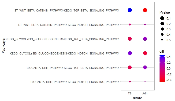
Above dot plot shows cooccurence of different pathway pairs in different cell types.
Continuum score for pathways on minimum spanning tree
UniPath also helps in visualization of gradient of pathways on minimum spanning tree, thus showing lineage potency as well other properties such as tumorigenicity etc. We have included lung cancer data for the tutorial. In the example given below, we are converting lung cancer gene expression data into pathway scores and plotting minimum spanning tree. Using this minimum spanning tree we are showing gradient of GO_REGULATION_OF_ICOSANOID_SECRETION pathway using its ajusted p-value.
library(UniPath)

##Load Lung cancer data
data("human_null_model")
data("c5.bp.v6.0.symbols")
data("lungcancer_expression")

Pval = binorm(human_null_data)
combp_ref = combine(c5.bp.v6.0.symbols,human_null_data,rownames(human_null_data),Pval)
Pval1 = binorm(expression_matrix)
combp = combine(c5.bp.v6.0.symbols,expression_matrix,rownames(expression_matrix),Pval1)
scores = adjust(combp,combp_ref)

distclust = dist_clust(scores$adjpvalog,2)
dist = distclust$distance
clusters = distclust$clusters
index = index(scores$adjpvalog,5)
KNN = KNN(scores$adjpvalog,index,clusters)
class = class1(clusters,KNN)
distance = distance(dist,class,clusters)
corr_mst = minimum_spanning_tree(distance)

vertex_color  = c( 'green' , 'red')
cell_labels = data.frame(c(rep("NSCLC TS cells",80),rep("Adherent NSCLC cells",82)))
set.seed(50)
UniPath::mst.plot.mod(corr_mst, vertex.color = vertex_color[cell_labels[,1]],mst.edge.col="black",bg="white",layout.function="layout.kamada.kawai",v.size = 3,e.size=0.005,mst.e.size = 0.005)
legend("topright", legend = sort(unique(cell_labels[,1])) , col = vertex_color,pch=20, box.lty=0,cex=1,pt.cex=2,horiz=F)

##Showing gradient of a pathway on mst
set.seed(50)
coltri = gradient(scores$adjpva, "GO_REGULATION_OF_ICOSANOID_SECRETION")
UniPath::mst.plot.mod(corr_mst, vertex.color = coltri,mst.edge.col="black",bg="white",layout.function="layout.kamada.kawai",v.size = 4,e.size=0.005,mst.e.size = 0.005)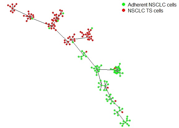
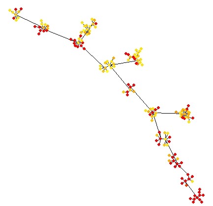
Above figure shows an increase in the gradient of a pathway in NSCLC TS cells.